Having not posted for over a year, I thought I would make a summary of what has been going on with the project since my last post. Not much progress or work was done at the beginning of the year. My bachelor’s thesis, together with other school projects, ended up taking much of my time. Some work was done to make sure that once summer came, I would be ready to continue working on the robot. When summer came, I transported my robot from my student room to my parents’ place in the countryside, an environment more suited for experimenting. Later in the year, I moved to Barcelona for my exchange studies. During my stay in Barcelona, I managed to make quite a lot of progress on the project, working mostly on an ML solution for the costmap problem, which I later wrote about.

---

First forestry test

Having only been able to perform small tests outside my student room on grass before, I was finally able to test the robot in forestry terrain, which is the environment it’s being built for.

However, a problem that appeared in this environment was the high friction force generated when trying to turn in the mossy terrain. When deciding the power of the motors and the gear ratio in the design phase, I had to make some guesses about what would be sufficient. This guess appeared to be somewhat too low. My plan is to fix this next year by getting bigger sprockets on the axes connected to the motors, doubling the torque but reducing the speed by half. It’s possible to see in the video, towards the end, me trying to turn the robot but struggling.

Later this summer, the DC driver had a transistor blow up on me when I tried to push the robot too much. The double-channeled driver on the robot is designed to have a maximum continuous current of 10A, with peaks of 30A for a few seconds. What I think happened was too many peaks in a short duration. Luckily for me, this happened later in the summer.

Mapping

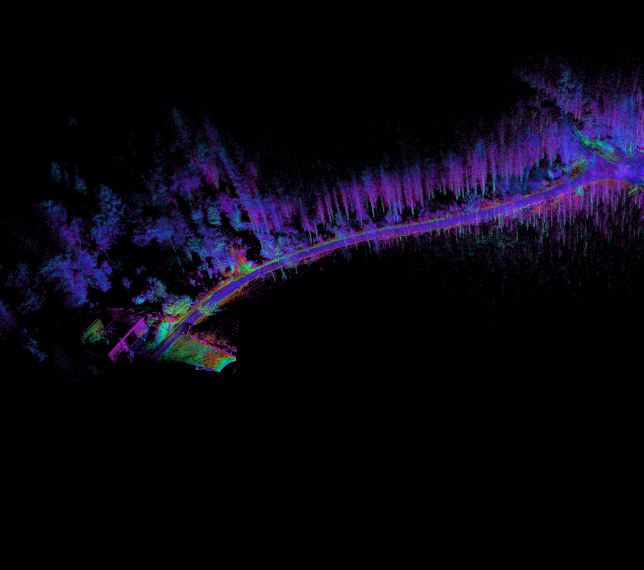
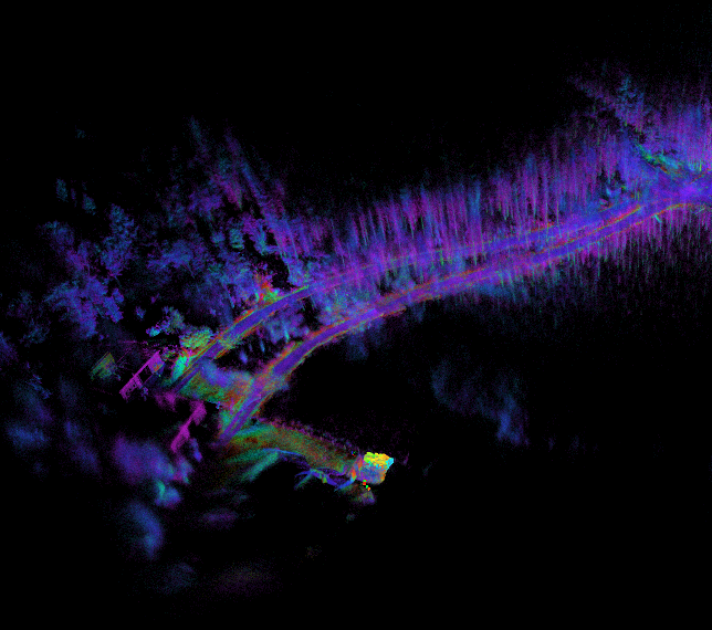
Ever since the start of the project, mapping an environment has been something I’m deeply fascinated by. I was able to achieve some success with the mapping. My test environment was a 500-meter-long gravel road in the forest where I drove back and forth.

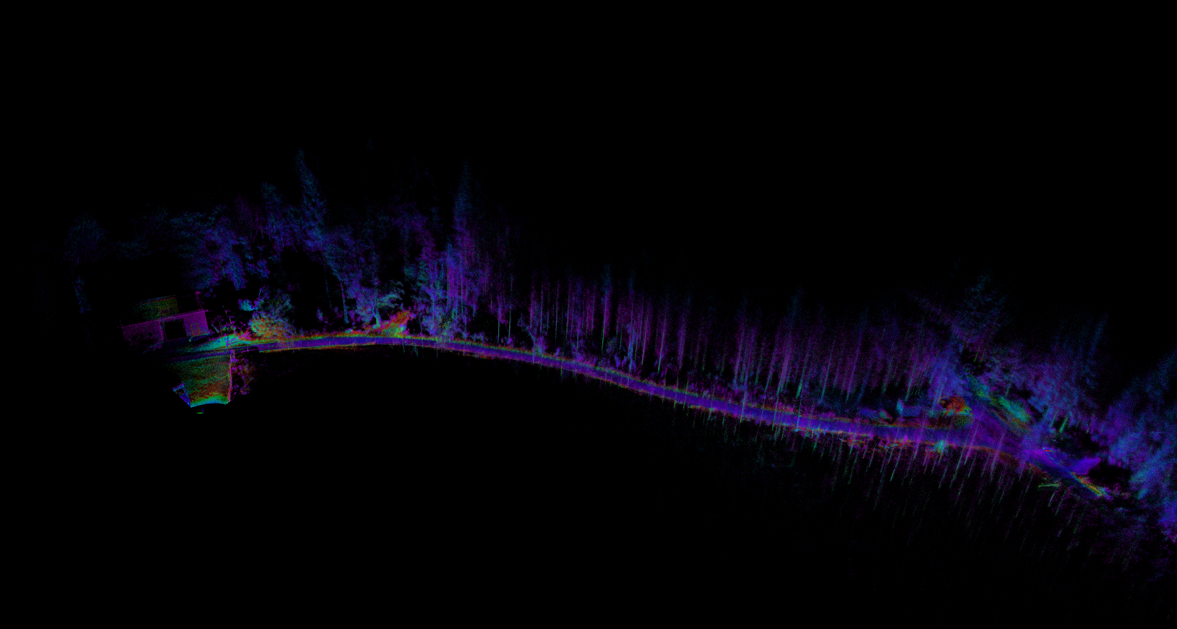
It was really cool seeing the forest I grew up with being built up in 3D on my screen. However, the mapping had some problems I had not foreseen.

Drift problem:

When performing the mapping, I experienced unwanted drift. Several times, the mapping lost its actual position, and instead of updating the map at the correct position with the new data, it updated at the wrong positions, creating a faulty map. This can be seen in the image below, where a new road is created on the way back, even though it’s the same road.

Possible explanations for the drift:

Something I never thought about during the build was that driving the robot would generate these kinds of vibrations. When the robot was running, and especially when turning on gravel, I experienced a lot of vibrations. The wheels are connected to the frame without any springs or dampening material. Because of this, everything felt by the wheels is transferred to the robot. The mapping uses data from both the Lidar and IMU, which makes me think that the vibrations are interfering with the mapping.

Resolution problem:

Something that I have come to realize more and more later this year is that the quality and resolution of the mapping are too low for what I plan to do in the future. This summer, all runs with the robot were controlled manually with a joystick. My future plans are to make it not only able to drive back and forth on a road like this but also in forestry terrain, as seen in the first video, fully autonomously. I realize that in order to have a chance of achieving this, I will need a much higher resolution of my surroundings.

From watching many hours of robot and mapping-related videos, I have seen what technology is currently available. I also now have a better understanding of what I need. The one sensor that stands out from the rest with regard to performance and price is the ZED2i RGB-D from Stereolabs. From what I can see, it appears to have the capability to generate a relatively high-resolution map with colors out of the box. I have been in contact with Stereolabs to try to obtain a larger dataset where I can evaluate the results. Unfortunately, they could not provide me with any dataset. Instead, they advised me to order one and use the 30-day free return option if I wasn’t satisfied.

I have now ordered one, and it’s expected to arrive in Sweden on the same day I return to Sweden for Christmas and New Year’s. Once I get it, I will try to perform some more challenging mapping trials and evaluate the results. Some of the things I will try are:

• Drift
• Large environment mapping
• Loop-closure

A demonstration video of mapping with the ZED2i can be seen bellow.

---

COSTMAP

However, when dealing with uneven terrain, there are other scenarios that need to be addressed. Here are a few:

• How can the robot understand that it can drive over a stump that fits under the robot, or over a smaller stone, but at the same time not collide with a stump or rock that is too big for the robot to drive over?
• In the forest, there are many slopes and even holes. How will the robot understand which slopes and holes it can drive over, so that it does not tip over or get stuck?
• Driving through obstacles could sometimes be allowed. How can the robot know that it can drive through high grass or even some smaller bushes?

I have spent countless hours researching the topic of autonomous navigation in uneven terrain, ever since the start of the project. There are several research papers that claim to have ‘solved’ this. Most of them do so by implementing some algorithm, and usually, the terrain is not too difficult. Nowhere did I find something that was well documented and that I thought would solve my problem. Feeling somewhat disappointed, I thought, ‘Let’s solve it with machine learning, as everyone else seems to be doing this year.

First attempt -> Reinforcement learning

Proximal policy optimization

Not having too much knowledge about the implementation of machine learning, I thought that reinforcement learning would be a good start. A few years ago, I had tried the PPO (Proximal Policy Optimization) algorithm over a weekend and decided to use it for my project, due to its robustness and easy implementation. Below are some concepts for my environment that are needed to understand.

• 3D True State: A 10x10x10 space that represents the ground truth of an area.
• 3D Current State: A 10x10x10 space fed to the model that represents the current mapping of the ground truth, where each element represents a point in a point cloud.
• Action: The current output for the cost map based on the current state.
• Last Costmap: The last output from the model, used to compare the change from the current one.
• True Costmap: The correct cost map generated from the true state, used to check the correctness of the outputted cost map.

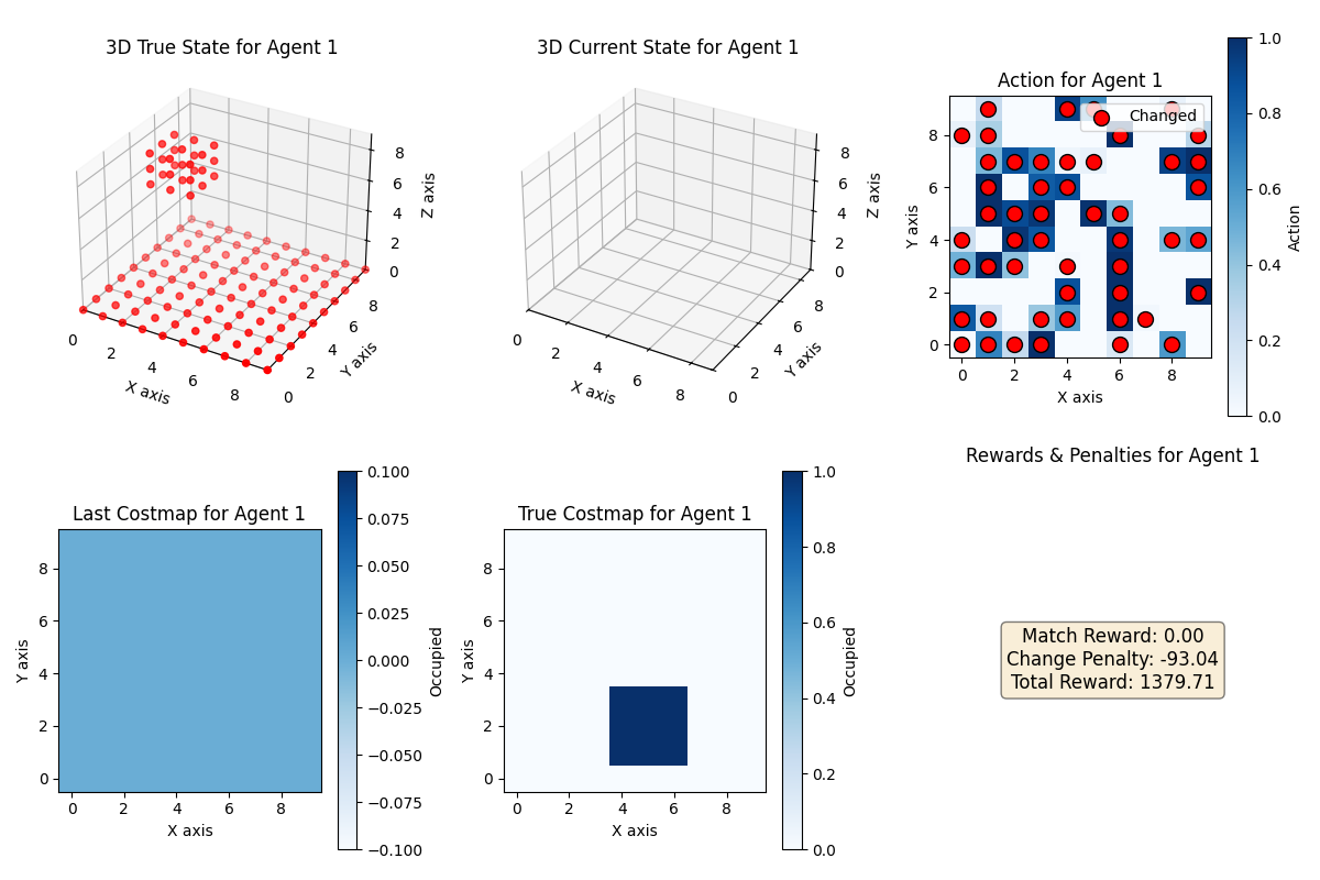
Environment setup

The model worked by first generating a 3D ground truth that would represent a space in an environment. The idea was to later use a much bigger space, like 100x100x100, where each element would represent a cubic centimeter, and the data gathered from a real mapping. In this case, a randomly sized cube was placed randomly inside the space, representing an obstacle by setting those positions as true. Also, all z = 0 positions were set to true to simulate the ground. From this space, a 10×10 ground truth cost map was generated, setting all values under the cube to 1, representing high cost.

Reward functions

The way RL works is by simulating steps. For each step, the model gets fed an input, which in my case was the current state. Based on this input, the model generates a cost map. The model would then get a reward for this output, depending on how I would reward it. For the first step, when the current state was empty, I would reward it extra for generating a cost map with a lot of free space, trying to promote it to prefer making an area free instead of occupied. I would then, for each step forward, insert one new random point from the true state and reward it for being close to the ground truth cost map.

Results

I ran different experiments on this setup, implementing CNNs and running the model with hundreds of different hyperparameters for millions of steps, even giving the model many new points each step. But experimenting with this for two months taught me a lot, though I was never able to generate a model that gave me the results I wanted. This led me to try a more traditional approach by attempting to solve it with ‘regular machine learning’.

---

Second attempt -> Machine learning

As I write this, I have actually only spent close to the last 2-3 weeks working on this approach. But it looks like this approach could actually solve my cost map problem. Instead of calculating the reward and having a state as in RL, I only feed my model with the fully mapped 10x10x10 state, together with my expected cost map output.

Update

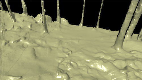
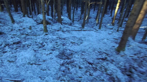
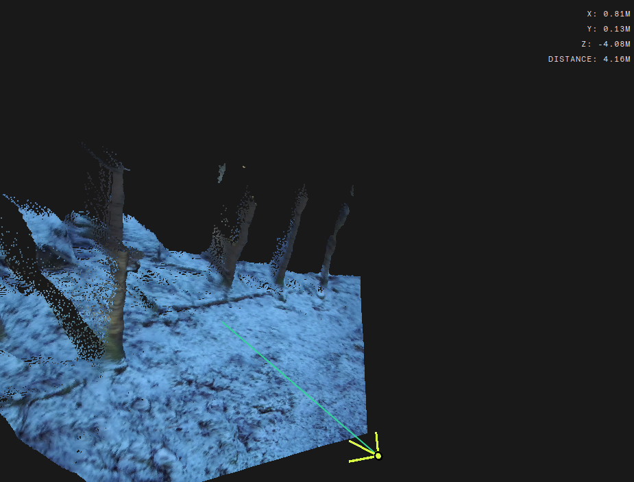
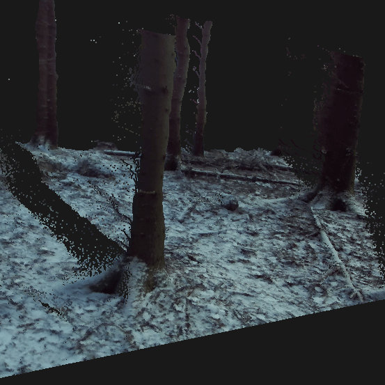
During my short stay in Sweden over Christmas, I got my hands on the ZED2i. I only had a few days to gather data and run experiments. My initial plan was to use the data from the mapping to generate a cost map; however, I learned something interesting while experimenting. Since the ZED2i has an IMU internally and knows the depth for each pixel, it can calculate and output 3D positions for each pixel in the RGB image in relation to the camera. This made me think of using the mapping only to know my current position in an environment, and then using the RGB image together with the depth image to generate cost values for positions based on my current location. I created a model that, with very little data, was able to output trees as obstacles with quite good results. Once I get back to Sweden in January, I will gather more data and generate a better model that hopefully will be able to accurately detect all obstacles in the environment, not just trees. I hope this method will result in solving the cost map problem in 2025. Below are some images showing the data outputted by the camera. In the last image, in the top right corner, you can see the positions of the selected pixel.